Introduction
Ever since I have read the refresher of Tjalling Jager on differential equations and likelihood functions, I have been irritated about the common way to express the likelihood of data following a normal distribution using the density function of the normal distribution. The statement that made me wonder was "note that we have seamlessly gone from probabilities to probability densities; this should not concern us here" (p. 23).
It seemed to me that the likelihood should rather be expressed as the integral of the probability density over the interval that is covered by a certain representation of a numeric value. For example, if an observation was reported to be "1.2", the associated interval would range from 1.15 to 1.25.
Only recently, when reading in the documentation of the mlt package by Hothorn (2018), I noticed that a similar argument about the approximation of the likelihood of continuous random variables has been mad earlier (Lindsey, 1999).
The case of a single observation ...
In order to put the interval idea to work, we start with a single observation. For a continuous random variable $Y$ with a known normal distribution, the probability of a single observation to be within the interval $] \underline{y}, \overline{y} ]$ is
$$ \mathbb{P}(\underline{y} < Y \le \overline{y} \mid \mu, \sigma) = \Phi\left(\frac{\overline{y} - \mu}{\sigma}\right) - \Phi\left(\frac{\underline{y} - \mu}{\sigma}\right) $$
Using our example of an observed value of 1.2, assuming that it implicitly means that the true value is in the interval ]1.15,1.25], we can define a function to calculate this probability in R as:
prob_obs <- function(lower, upper, mean = 0, sd = 1) {
  pnorm(upper, mean, sd) - pnorm(lower, mean, sd)
}
(p_1.2 <- prob_obs(1.15, 1.25))
[1] 0,01942216
log(p_1.2)
[1] -3,94134
The probability of this observation, assuming a standard normal distribution for the underlying statistical population is obtained to be about 0,0194, which is very close to the probability density at the value of 1.2 times the width of the interval. If we simply approximate the probability by the probability density, the factor by which this is off (and thus the shift in the log-likelihood) will depend on the units chosen for the observation.
Note that we have not distinguished between inclusive and exclusive bounds of the interval, as the numeric representation of the bounds in R will generally be of sufficient precision so that the difference between the closest match to a bound (e.g. 1.15) and the next possible value can be considered negligible for this analysis.
In order to obtain the parameters of the normal distribution that is most consistent with our observation, we can then proceed to interpret the probability of the observation given above as the likelihood of the model parameters
$$ L(\mu, \sigma | y) = \mathbb{P}(\underline{y} < Y \le \overline{y} \mid \mu, \sigma) $$
and maximise it to obtain maximum likelihood estimates (MLE) $\hat{\mu}$ and $\hat{\sigma}$ for the distribution parameters by minimizing the negative log-likelihood.
log_lik <- function(mean, sd, data) {
  sum(log(prob_obs(data$lower, data$upper, mean, sd)))
}
objective <- function(theta, data) {
  - log_lik(theta["mean"], theta["sd"], data)
}
min_1.2 <- nlminb(start = c(mean = 0, sd = 1),
  objective, data = data.frame(lower = 1.15, upper = 1.25),
  lower = c(mean = -Inf, sd = 0),
  control = list(trace = 1))
  0:     3,9413405:  0,00000  1,00000
  1:     3,5358156: 0,939180  1,34343
  2:     3,0483807:  1,41780 0,810734
  3:     2,9329842:  1,39233 0,722755
  4:   0,014035847:  1,19062 0,0183273
  5:    -0,0000000:  1,22768  0,00000
  6:    -0,0000000:  1,22768  0,00000
print(min_1.2$par)
    mean       sd
1,227683 0,000000
We see that the optimization converges to a mean somewhere in the specified interval and a standard deviation of zero.
In order to better understand this result, we can visualize the likelihood profile:
mu_plot = seq(1, 1.4, by = 0.01)
sigma_plot = seq(0, 0.4, by = 0.01)
z <- outer(mu_plot, sigma_plot,
  function(mean, sd) prob_obs(1.15, 1.25, mean, sd))
persp(mu_plot, sigma_plot, z,
  theta = 35, phi = 20, ticktype = "detailed",
  xlab = "Mean", ylab = "Sigma", zlab = "Likelihood")
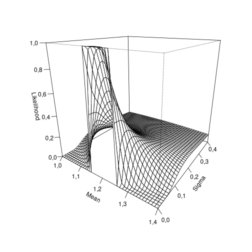
plot of chunk profile
Thus our model suggests that the most likely normal distribution given our single observation has a standard deviation close to zero and a mean somewhere in the interval between 1.15 and 1.25.
Several, potentially censored observations
In order to conveniently deal with several such observations, we define a function that converts certain character representations of our observations into a dataframe containing the lower and upper bounds of the corresponding observational intervals. Also, we want to be able to specify left and right censored observations using representations like '< 0.2' or '> 5.0'.
as.obs <- function(x) {
  if (any(sapply(x, function(a) grepl("e", a)))) stop ("Scientific notation is not supported")

  left <- grepl("^<", x)
  right <- grepl("^>", x)
  x_num <- as.numeric(gsub("^[<>]", "", x))
  decimals <- gsub(".*\\.", "", x)
  n_decimals <- nchar(decimals)
  interval_range <- 10^-n_decimals
  lower <- ifelse(left, -Inf, ifelse(right, x_num, x_num - 0.5 * interval_range))
  upper <- ifelse(right, Inf, ifelse(left, x_num, x_num + 0.5 * interval_range))
  ret <- data.frame(lower, upper)
  return(ret)
}
x <- c("1.2", "3.273", "< 0.2", "> 2.7")
x_obs <- as.obs(x)
print(x_obs)
   lower  upper
1 1,1500 1,2500
2 3,2725 3,2735
3   -Inf 0,2000
4 2,7000    Inf
We can now estimate the parameters of the supposed underlying normal distribution and calculate the log-likelihood of the solution.
min_x_obs <- nlminb(start = c(mean = 0, sd = 1),
  objective, data = x_obs,
  lower = c(mean = -Inf, sd = 0),
  control = list(trace = 1))
  0:     23,334776:  0,00000  1,00000
  1:     16,546212: 0,351102  1,93634
  2:     15,687217:  1,31191  1,73492
  3:     15,636878:  2,14422  1,56714
  4:     15,517024:  1,74168  1,70304
  5:     15,494396:  1,77305  1,73891
  6:     15,422965:  1,88078  1,96280
  7:     15,412944:  1,90232  2,06494
  8:     15,411206:  1,90644  2,12210
  9:     15,411132:  1,90409  2,13473
 10:     15,411128:  1,90225  2,13624
 11:     15,411127:  1,90111  2,13621
 12:     15,411127:  1,90094  2,13602
 13:     15,411127:  1,90094  2,13598
print(min_x_obs$par)
    mean       sd
1,900940 2,135979
log_lik(min_x_obs$par["mean"], min_x_obs$par["sd"], x_obs)
[1] -15,41113
In order to check what we have done, we can do the same using the survreg function in the survival package. At this point I would like to thank Torsten Hothorn for pointing out that this is possible and how it is done.
library(survival)
x_Surv <- Surv(x_obs$lower, x_obs$upper, type = "interval2")
x_survreg <- survreg(x ~ 1, data = data.frame(x = x_Surv), dist = "gaussian")
summary(x_survreg)
Call:
survreg(formula = x ~ 1, data = data.frame(x = x_Surv), dist = "gaussian")
Warning in printCoefmat(x$table, digits = digits, signif.stars = signif.stars,
: NAs introduced by coercion
            Value Std. Error    z     p
(Intercept) 1,901      1,144 1,66 0,097
Log(scale)  0,759      0,567 1,34 0,181

Scale= 2,14

Gaussian distribution
Loglik(model)= -15,4   Loglik(intercept only)= -15,4
Number of Newton-Raphson Iterations: 4
n= 4
Voilá, we obtain the same results for the distribution parameters as well as for the log-likelihood!
Comparison with fitdistrplus
The package fitdistrplus also provides a way to fit distributions to censored data, namely via the fitdistcens function. However, the package vignette gives a likelihood function that mixes probabilities and probability densities. We can assess the effect of this in our example case. At first, we use the same interpretation of the observed data that we have used above.
library(fitdistrplus, quietly = TRUE)
x_censdata <- data.frame(
  left = ifelse(x_obs$lower == -Inf, NA, x_obs$lower),
  right = ifelse(x_obs$upper == Inf, NA, x_obs$upper))

x_fitdistcens <- fitdistcens(x_censdata, "norm")
summary(x_fitdistcens)
Fitting of the distribution ' norm ' By maximum likelihood on censored data
Parameters
     estimate Std. Error
mean 1,901758   1,144381
sd   2,136302   1,211426
Loglikelihood:  -15,41113   AIC:  34,82226   BIC:  33,59484
Correlation matrix:
           mean         sd
mean 1,00000000 0,01217819
sd   0,01217819 1,00000000
As expected, we get pretty much the same results here as well. However, if we interpret the simple observations as exact (or non-censored) observations, we obtain a slightly different picture.
x_partcens <- data.frame(
  left = c(1.2, 3.273, NA, 2.7),
  right = c(1.2, 3.273, 0.2, NA))
x_fitpartcens <- fitdistcens(x_partcens, "norm")
summary(x_fitpartcens)
Fitting of the distribution ' norm ' By maximum likelihood on censored data
Parameters
     estimate Std. Error
mean 1,901134   1,144231
sd   2,136102   1,211229
Loglikelihood:  -6,200705   AIC:  16,40141   BIC:  15,174
Correlation matrix:
           mean         sd
mean 1,00000000 0,01162075
sd   0,01162075 1,00000000
While the parameter estimates are, as expected, approximately the same, we do obtain a different value for the log-likelihood. Ronald A. Fisher, when he introduced the term likelihood, stated that there is no absolute measure of likelihood (Fisher and Russell, 1922). In fact, the term was introduced in order to avoid the necessity to be able to interpret it as a probability or "inverse probability". However, in view of potential further interpretations of the likelihood it seems prudent to use a consistent definition for the likelihood of each observation in a set of observations, which must be based on an integral of the underlying probability density in the presence of censored data.
Note added on 30 August 2021: From todays point of view, I would say that I was a bit naive to assume "potential further interpretations of the likelihood". But nevertheless, it seems to me that the use of integrals over probability densities may still give improved estimates if different accuracies are used in a set of observation, e.g. a higher absolute precision is used for small numbers than for large numbers. An example set of such observations would be (0.12, 0.41, 3.2, 15). In this example, it is obvious that different precisions are used and with the method sketched out above, this can be taken into account in the calculation of the likelihood of the data. Note that to be sure of such differences in precision they must be documented, as for example the number 3.2 could also be the result of sloppy notation (or formatting artefact) of an original reading of 3.20.
Bibliography
R. A. Fisher and Edward John Russell. On the mathematical foundations of theoretical statistics. Philosophical Transactions of the Royal Society of London. Series A, Containing Papers of a Mathematical or Physical Character, 222(594-604):309–368, 1922. URL: https://royalsocietypublishing.org/doi/abs/10.1098/rsta.1922.0009, doi:10.1098/rsta.1922.0009. ↩
Torsten Hothorn. Most likely transformations: the mlt package. Journal of Statistical Software, 2018. Accepted for publication 2018-03-05. URL: https://cran.r-project.org/package=mlt. ↩
J. K. Lindsey. Some statistical heresies. The Statistician, 48:1–40, 1999. ↩